Speech Emotion Recognition
1.Introduction
Speech is the primary tool used by humans to interact and convey information. But what type of information is really delivered? It is believed that speech is a tool to express not only thoughts but also emotions. Apart from linguistic messages that clearly express emotions, certain messages are ambiguous: The linguistic part does not define the emotion behind it. In this article we try to combine emotional prosody -non-verbal aspects of language that allow people to convey or understand emotion- and deep learning in order to create a model that understands human emotion through speech.
2.Dataset
In order to compensate the lack of data and generalize better, I created a dataset from 4 public datasets of speech emotion recognition.
- Toronto emotional speech set (TESS): a female only dataset with 7 classes
- RAVDESS Emotional speech audio: a dataset containing 1440 audio clip and 24 professional actors (12 female, 12 male).
- SAVEE Database: this dataset was recorded from four native English male speakers
- CREMA-D (Crowd Sourced Emotional Multimodal Actors Dataset): a dataset of 7,442 original clips from 91 actors. These clips were from 48 male and 43 female actors between the ages of 20 and 74 coming from a variety of races and ethnicities.
Our labels consist of 14 classes: 7 emotions divided by the gender (male female). The 7 emotions are anger, sadness, happiness, boredom, surprise, disgust and the neutral emotion.
At first glance, the data seems to be unbalanced, due to the presence of male only and female only datasets. However, these datasets were chosen precisely for their quality. In addition, joining four datasets was an important factor to fight back the imbalance.

3.Approach Overview
For this problem I chose a workflow consisting 3 major steps:
Step 1: Data augmentation
Although we are using 4 datasets and 10000 audio clips, creating a model from scratch needs a lot more data. Data augmentation seems critical in this problem in order to generalize better and for regularization purposes. Data augmentation might help the neural network extract more complex features from the data and avoid simpler features that may overfit the model.
Step 2: Feature extraction
In the context of emotional prosody, models tend to not comprehend the raw audio data. So I extracted the features that represent audio data, as we humans hear, and features that describe the audio data. The extracted features are MFCC, spectral rolloff, spectral centroid, spectral bandwidth, spectral rolloff and zero crossing rate.
Step 3: Modeling
I chose a combination of CNN and LSTM multi-input model with local attention for the most important audio features. For each feature, I apply CNN across the time dimension (convolution operations are applied for every timestep of the audio data) for feature extraction. The result passes to LSTM and fully connected layers to predict the right class. More details will be discussed in the modeling section.

4.Removing Noise
In this solution, the main goal is the creation of a model that generalizes predicting speech emotion. The majority of the audio clips of these datasets are clear, that why it is crucial to deal with the noise coming from poor mics. To tackle this problem, I tried to apply an envelope function, a function that divides the audio data in windows. If the volume mean value in the window is under a certain threshold, the audio part related to the window will be discarded.
5.Data Augmentation
My aim for data augmentation is to augment the data without changing the labels and to diversifying the data.
Pitch change: I choose this type of augmentation because although it seems that pitch changes may be impactful on the emotion, the pitch was shifted minimally to not affect the labels and to insist on the fact that pitch doesn’t define the gender. This augmentation is really helpful for regularization purposes.
Speed change: The speed change augmentation was used to generate more data without affecting the audio.
Value augmentation: The audio data was multiplied by a uniform distribution in order to generate more data without affecting the nature of audio
Adding Noise: Noise is always apparent in real-life recordings. The noise remover method used is only partial and doesn’t radically solve the issue, so adding noise as an augmentation tool might help to generalize better. I choose to add the Gaussian distribution to the audio data.
6.Audio Feature Extraction
This part is where things get spicy. There are a ton of audio Features that can be extracted from audio data and their use depends on the problem. My main focus is on features that represent the audio energy pitch loudness. I stuck with spectral features that seemed to convey information about human emotions.
MFCC (Mel-frequency cepstral coefficients): The MFCC is one of the main features that are used with audio models. They are quite popular with this type of problem due to the fact that they approximate the human auditory system’s response, unlike linearly-spaced frequency bands.
Spectral rolloff: Spectral rolloff is the frequency below which a specified percentage of the total spectral energy (0.85 used in our case). It gives an idea about how high frequencies are getting.
Spectral centroid: The spectral centroid indicates at which frequency the energy of a spectrum is centred upon. This feature resembles the attention mechanism applied on feature extraction. It can be helpful for the model to understand which part of the audio to focus on, the most.
Zero-crossing rate (ZCR): The zero-crossing rate is the rate of sign-changes along a signal (in both ways (positive-negative, negative-positive). This feature is helpful to understand when a human is speaking (Voice activity detection).
Root-mean-square energy (RMSE): This feature as its name indicates is responsible of extracting energy values along a signal.
Spectral bandwidth: Spectral bandwidth is the wave-length interval in which a radiated spectral quantity is not less than half its maximum value. It is basically a measure of the extent of the Spectrum.
7.Modeling
Time distributed Layers:
The modeling approach consists of considering the coefficients of the features as a one-dimension images. In this case CNN seems like a reasonable approach to solve the problem. Indeed it is, however something is missing. Every input contains several images that are chronologically ordered. So, we need the input as a sequence of images on which we apply convolutional operations. This is where the time distributed layers come in handy. They basically solve this specific issue. When applied to a child layer, the time distributed layer will apply the operations of the child layer on each frame (each image in our case).
The advantage of this layer is that the weights are trained together in the back propagation (the same backward pass), this way, the weights are updated by analysing the whole sequence.
Attention:
Attention is basically a mechanism by which a network can weigh features by level of importance to a task, and use this weighting to help achieve the task. Which means that considering certain features in our system (neurons in the case of neural networks), we assign a weight for each feature to neglect unwanted information and to focus on important parts of the network.
We can use two types of attention: soft and hard. In our case we worked with soft attention which means that I multiply this attention map over the selected layer to get weighted features.
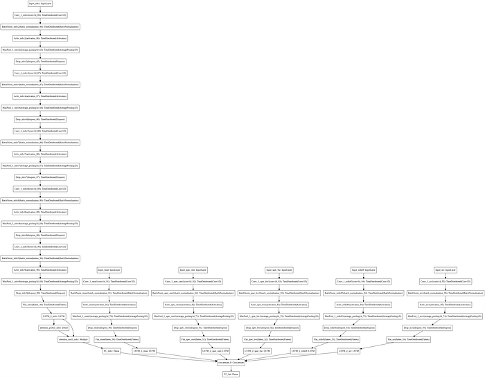
The model architecture:
The model consists of 3 phases:
Phase 1: Time distributed convolution layers
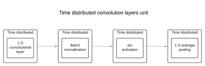
We apply time distributed convolutional layers on each spectrogram in order to extract information. In this phase, a time distributed convolutional layers unit contains:
- Time distributed 1D convolution layer
- Time distributed batch normalization
- Time distributed elu activation
- Time distributed 1D Average pooling (average pooling gave better results than max pooling)
The number of times this unit is applied depends on the feature.
After applying these units we finally apply a time distributed flatten layer to prepare for the next phase.
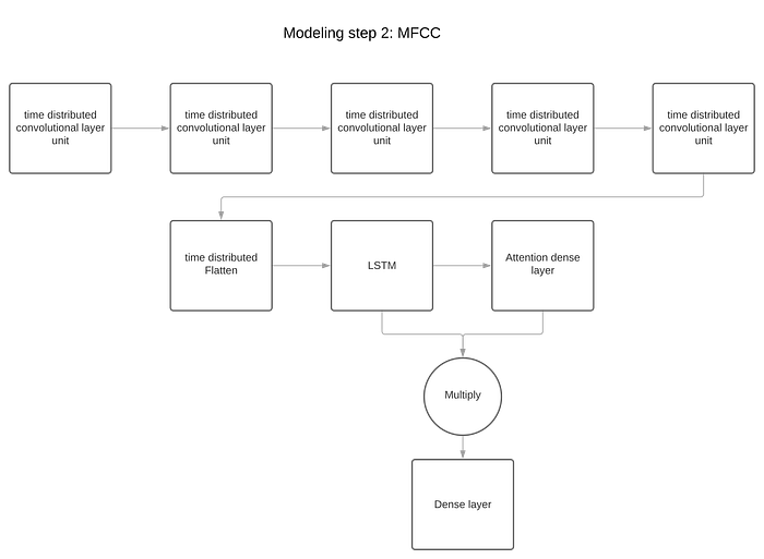
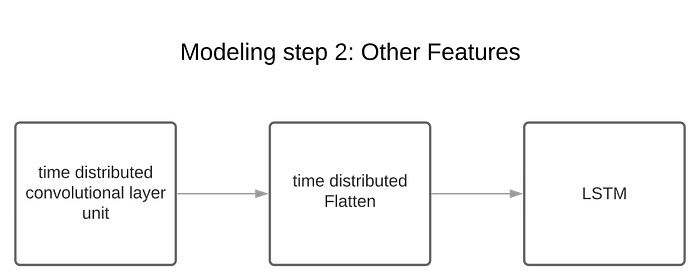
Phase 2: LSTM + local attention
In this phase, we apply LSTM (long short term memory) which is a recurrent structure that helps memorize patterns for long term which is beneficial in our case (We need to work with the whole sequence). In this layer the output is the last unit of the sequence not the whole sequence (sequence to one).This layer is applied on each feature. For MFCC, I added a local attention mechanism after the LSTM layer
MFCC schema:
Other features schema:
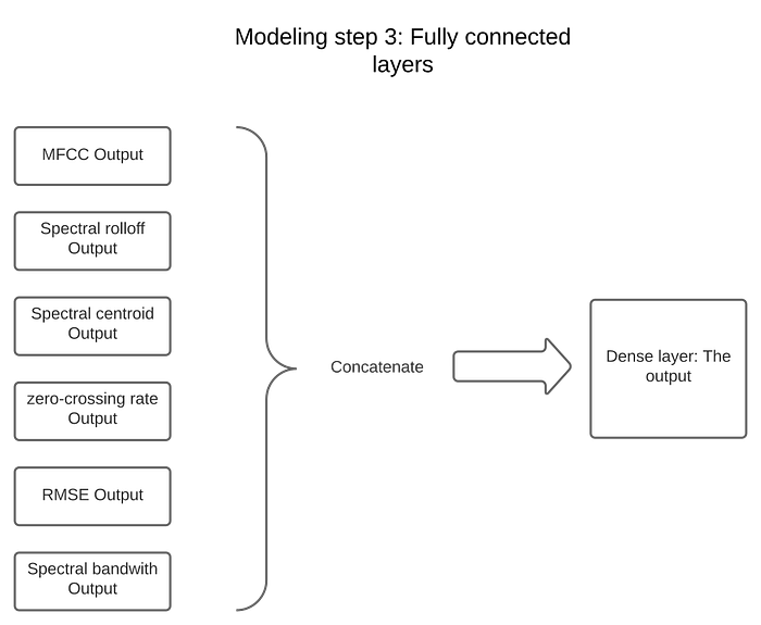
Phase 3: Fully connected layers
After applying LSTM on all the features, the results are concatenated in a dense layer and fed into fully connected layers. The output is the classification decision.
The model was trained with 64 batch size with the default adam as optimizer and categorical cross entropy as loss
8.Results, Interpretations and Notes:
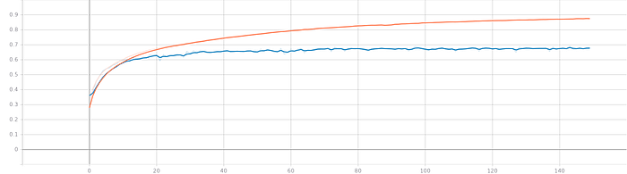
I mainly choose the best model based on validation accuracy. Here are the results after 200 epochs of training.
Accuracy plot :
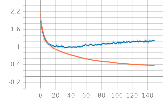
Loss plot:
Some stats for each class:
class : male_angry accuracy : 0.77 precision 0.64 recall 0.77
class : male_disgust accuracy : 0.48 precision 0.56 recall 0.48
class : male_fear accuracy : 0.49 precision 0.64 recall 0.49
class : male_happy accuracy : 0.42 precision 0.45 recall 0.42
class : male_neutral accuracy : 0.77 precision 0.59 recall 0.77
class : male_sad accuracy : 0.59 precision 0.55 recall 0.59
class : female_angry accuracy : 0.87 precision 0.78 recall 0.87
class : female_disgust accuracy : 0.63 precision 0.72 recall 0.63
class : female_fear accuracy : 0.74 precision 0.74 recall 0.74
class : female_happy accuracy : 0.72 precision 0.84 recall 0.72
class : female_neutral accuracy : 0.84 precision 0.75 recall 0.84
class : female_sad accuracy : 0.76 precision 0.71 recall 0.76
class : male_surprise accuracy : 0.50 precision 0.82 recall 0.50
class : female_surprise accuracy : 0.94 precision 0.98 recall 0.94
It seems that the model is having a hard time identifying emotions for males. Separating the 2 genders might improve the results and should be tried out in the next phases
It seems that the model is overfitting on the training data at the end. 69% overall seems a great result, considering the model is trained from scratch and the data isn’t homogeneous.
The attention mechanism did not affect the result too much but it improved it a bit so I decided to keep it.
I tried the MEL spectrogram instead of MFCC, but it costs too much computational power and the results were worse so I dropped it.
Even with these results, generalizing the model seems to be far ahead. It needs more data and more computational power.
GitHub Link:
https://github.com/Mo5mami/SER
9.Final Thoughts:
There are a lot of ways to improve this approach overall, Data augmentation and dealing with noise might do it with more complex ideas. Also, I may consider extracting more features from the audio. All of these will be considered in the next steps to improve the model and generalize better. On the good side, although a lot of work still has to be done, this approach overall seems promising and it might be combined with other types of data (images videos text …) for multimodeling purposes.
Credits:
This project was developed within our Engineering Department, by Mokhtar Mami. Our amazing member wrote this article, also .
Email address: mami.mokhtar123@gmail.com